4.4 The Fundamental Theorem of Calculus
Lesson date: February 19, 2025.
- Evaluate a definite integral using the Fundamental Theorem of Calculus.
- Understand and use the Mean Value Theorem for Integrals.
- Find the average value of a function over a closed interval.
- Understand and use the Second Fundamental Theorem of Calculus.
Assignment
- Vocabulary and teal boxes
- p326 5–25 odd, 29, 32, 35–39 odd, 44, 45, 48, 50, 59, 65, 67, 70–72, 75, 76, 79 80, 83, 84, 89–91
Additional Resources
- AP Topics: 6.1, 6.4, 6.5, 6.6, 6.7, 8.1, 8.3
- Khan Academy
- Exploring accumulations of change
- The fundamental theorem of calculus and accumulation functions
- Interpreting the behavior of accumulation functions involving area
- Applying properties of definite integrals
- The fundamental theorem of calculus and definite integrals
- Finding the average value of a function on an interval
- Using accumulation functions and definite integrals in applied contexts
The Fundamental Theorem of Calculus
Disclaimer: The fundamental theorem of calculus has two parts. Our book goes through the two parts in the opposite order of most other sources. I am sticking with what everyone else does as I think it’s the easier way to grasp the concept.
And for clarification, here is how the two parts are referenced in different sources. I’ll try to use the AP names to avoid complication.
Book AP Course Description Everywhere Else Second Accumulation (6.4) First First Definite Integral (6.7) Second
The Accumulation Part
Let’s create a function, $A(x)$, that will produce the area under a curve, but $x$ will be the right bound of the interval. These area functions are also called accumulation functions since the area accumulates as $x$ increases.
Now, what if we increased that area and wanted to find out how much it increased? This is represented by the red strip in the image below. You start off with some set amount of area $A(x)$ (which is the blue area), and we want to just slightly move to the right $h$ units.
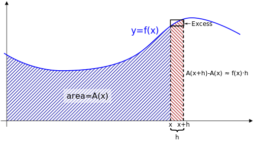
That would make the new area $A(x+h)$. Since we’re just interested in the change in area, the new area, we can subtract what was there to begin with, so $A(x+h) - A(x)$.
We can also estimate that area as a rectangle. The width is $h$ and we can use $f(x)$ as our height, because this is just an estimation. There is some amount of excess to account for, so we shouldn’t forget about it.
\[\begin{align} f(x) \cdot h + \text{Excess} \end{align}\]Well, that’s two different ways of expressing the same area, so we can set them equal to each other.
\[\begin{align} f(x) \cdot h + \text{Excess} = A(x+h) - A(x) \end{align}\]Rearranging, and accounting for the fact we want $h$ to be as small as possible, we get
\[\begin{align} f(x) = \lim_{h \to 0} \left(\frac{A(x+h) - A(x)}{h} + \frac{\text{Excess}}{h}\right) \end{align}\]That excess term will go to zero as $h \to 0$, so we ultimately end up with
\[\begin{align} f(x) = \lim_{h \to 0} \frac{A(x+h) - A(x)}{h} \end{align}\]Well, the right-hand side is literally the definition of a derivative.
\[\begin{align} f(x) &= A'(x) \label{eq:1}\\ F(x) &= A(x) \label{eq:2} \end{align}\]Recall that in this situation, $f(x)$ was the curve and $A(x)$ is the area under that curve. So, if the derivative of an area function is its original function (equation $\ref{eq:1}$), that means the area function is equal to the antiderivative of the original function (equation $\ref{eq:2}$). This is commonly known as the first part of the fundamental theorem and can be expressed a couple of different ways.
First Fundamental Theorem of Calculus (Accumulation)
\[\begin{align} F(x) = \int_a^x f(t) \, dt \label{eq:fun-1a} \\[1em] \frac{d}{dx}\left[\int_a^x f(t) \, dt \right] = f(x) \label{eq:fun-1b} \end{align}\]
First thing to note is the use of $t$ as the variable of integration. This is only done since $x$ is already in use as the upper limit of integration.
Also, the beginning of the interval doesn’t make it over to the other side. It’s a bit easier to picture in equation \ref{eq:fun-1b}. Since the derivative of the integral shows you how the area is changing (accumulating) at $x$, where the interval begins is irrelevant.
The Definite Integral Part
Now we can take idea behind the first part and apply it an area with constant endpoints, our definite integrals. We’ll need two accumulation functions though, since we’ll have to subtract them to find the area of the interval in question. We’ll also drop the $t$ since we don’t have $x$ in the interval anymore.
\[\begin{align} \int_a^b f(x) \, dx &= \int_0^b f(x) \, dx - \int_0^a f(x) \, dx \\[1em] &= F(b) - F(a) \end{align}\]This gives us the second part of the theorem. To find the area under a curve, evaluate the antiderivative of the upper bound minus the antiderivative of the lower bound.
Second Fundamental Theorem of Calculus (Definite Integral)
\[\begin{align} \int_a^b f(x) \, dx &= F(b) - F(a) \end{align}\]
Evaluating Definite Integrals
Applying the fundamental theorem is straightforward, provided you can come up with the antiderivative.
\[\begin{align} \int_1^2 (x^2-3)\,dx &= \left[ \frac{x^3}{3} - 3x \right]_1^2 \\ &= \left(\frac{8}{3}-6\right)-\left(\frac{1}{3}-3\right) \\ &= \left( \frac{7}{3}-3 \right) \\ &= -\frac{2}{3} \end{align}\]It’s sometimes helpful to work with similar terms when doing the arithmetic at the end. Above, I combined the $8/3$ and $1/3$, while combining the integer terms.
Integrals involving absolute values require an extra step since there is no antiderivative rule for them. Instead, find the vertex and split the integral into two, one for each part of the absolute value.
To find that split, set your absolute value equal to $0$. The reason for this is that the original vertex has an $x$ value of $0$, so we are looking for how to undo any transformation applied to it.
\[\begin{align} \int_0^2 |2x-1|\,dx &= \int_0^\frac{1}{2} -(2x-1)\,dx + \int_\frac{1}{2}^2 2x-1\,dx \end{align}\]The Mean Value Theorem for Integrals
When we first started estimating area with rectangles, we saw overestimates with one endpoint and underestimates with the other. From that, we can assume that there must be some point in the middle that would give us a correct value.
So, given an interval $[a,b]$, there must exist some $c$ that would produce the exact height needed to accurately calculate the area.
Mean Value Theorem for Integrals
\[\begin{align} \int_a^b f(x) \, dx = f(c) \cdot (b-a) \end{align}\]
Average Value of a Function
The average value of a function on an interval can be thought of two ways.
- Add up all the $y$ values on the interval and divide by how many (infinite in this case). The book has a proof of how this summation equals what we have in equation $\ref{eq:average}$.
- Take the area for that interval and reshape it into a rectangle with the same width as the interval. Its height is the average value.
If point 2 isn’t convincing, imagine the ocean with all the waves flattened out and you would have sea level.
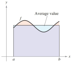
It turns out that the mean value theorem for integrals produced the average for us already: $f(c)$. That value, when multiplied by the interval, gave us the exact same area we started with.
Average Value of a Function
\[\begin{align} \frac{1}{b-a} \int_a^b f(x) \, dx \label{eq:average} \end{align}\]
Accumulation Functions and the Chain Rule
In the accumulation functions we’ve seen so far, we had $x$ as an upper bound. Complications arise when the upper bound is no longer just $x$. The chain rule can solve this problem, as all you need to do is derive like normal, but then multiply by the inner function. So, continue to substitute the upper bound in for $t$, but remember to multiply by its derivative at the end.
\[\begin{align} \frac{d}{dx} \left[ \int_{\pi/2}^{x^3} \cos t \, dt \right] = \left( \cos x^3 \right) \left( 3x^2 \right ) \end{align}\]