1.6 Linear Systems
A system of linear equations is a set of two or more equations using the same variables. The solution to a system is all the coordinates that make each equation true. In the event that a system doesn’t have a solution, it’s called an inconsistent system. Aside from graphing the system, similar to last section, you can typically solve systems through either substitution or elimination.
Substitution
Substitution is the more straightforward method, but not always practical.
\[\begin{align*} x + 2y &= 3 \\ x - 2y &= 4 \end{align*}\]You can rearrange both equations, solving for $x$.
\[\begin{align*} x &= 3 - 2y \\ x &= 4 + 2y \end{align*}\]If they are both equal to $x$, then they are equal to each other.
\[\begin{align*} 3 - 2y &= 4 + 2y \\ -4y &= 1 \\ y &= -\frac{1}{4} \end{align*}\]And with $y$ solved, we can plug back into either equation to find the value of $x$.
\[x = 4 + 2\left(-\frac{1}{4}\right) = \frac{7}{2}\]Elimination
Elimination involves performing operations to the equations in order to eliminate a variable. The operations are typically scaling, which is multiplying a equation by some constant, or adding/subtracting one equation from another.
See if you can follow what happens from one step to next. Each operation is one of the two listed above: scaling or adding another equation.
\[\left\{ \begin{aligned} 2x + y &= -1 \\[0.5em] -6x + 5y &= 7 \end{aligned}\right. \quad \Rightarrow \quad \left\{ \begin{aligned} 6x + 3y &= -3 \\[0.5em] -6x + 5y &= 7 \end{aligned}\right. \quad \Rightarrow \quad \left\{ \begin{aligned} 8y &= 4 \\[0.5em] -6x + 5y &= 7 \end{aligned}\right. \quad \Rightarrow \quad \left\{ \begin{aligned} y &= \frac{1}{2} \\[0.5em] -6x + 5y &= 7 \end{aligned}\right.\]Like before, we can substitute back into one of the original equations to find the value of the other variable.
\[\begin{align*} 2x + \frac{1}{2} &= -1 \\[1em] 2x &= -\frac{3}{2}\\[1em] x &= -\frac{3}{4} \end{align*}\]Systems of Inequalities
Solutions to systems of inequalities are typically best expressed as graphs. The combinations of solutions can be complex, so a picture of where they can be found is the most helpful
The book has an example with someone earning \$20 an hour mowing lawns and \$10 an hour walking his neighbors’ dogs. The catch is they can only work 20 hours a week, with at least 5 of that dedicated to dog walking, and he wants to make \$200 in a week.
We can relate the hours together, but also need to account for the dog walking minimum. That gives us
\[\begin{align*} m + d &\le 20\\ d &\ge 5 \end{align*}\]And we can relate the money as well. The hours worked multiplied by the rate gives us totals we can use with the \$200 he wants to make.
\[\begin{align*} 20m + 10d &\ge 200 \\ m + d &\le 20\\ d &\ge 5 \end{align*}\]When graphed, we get this
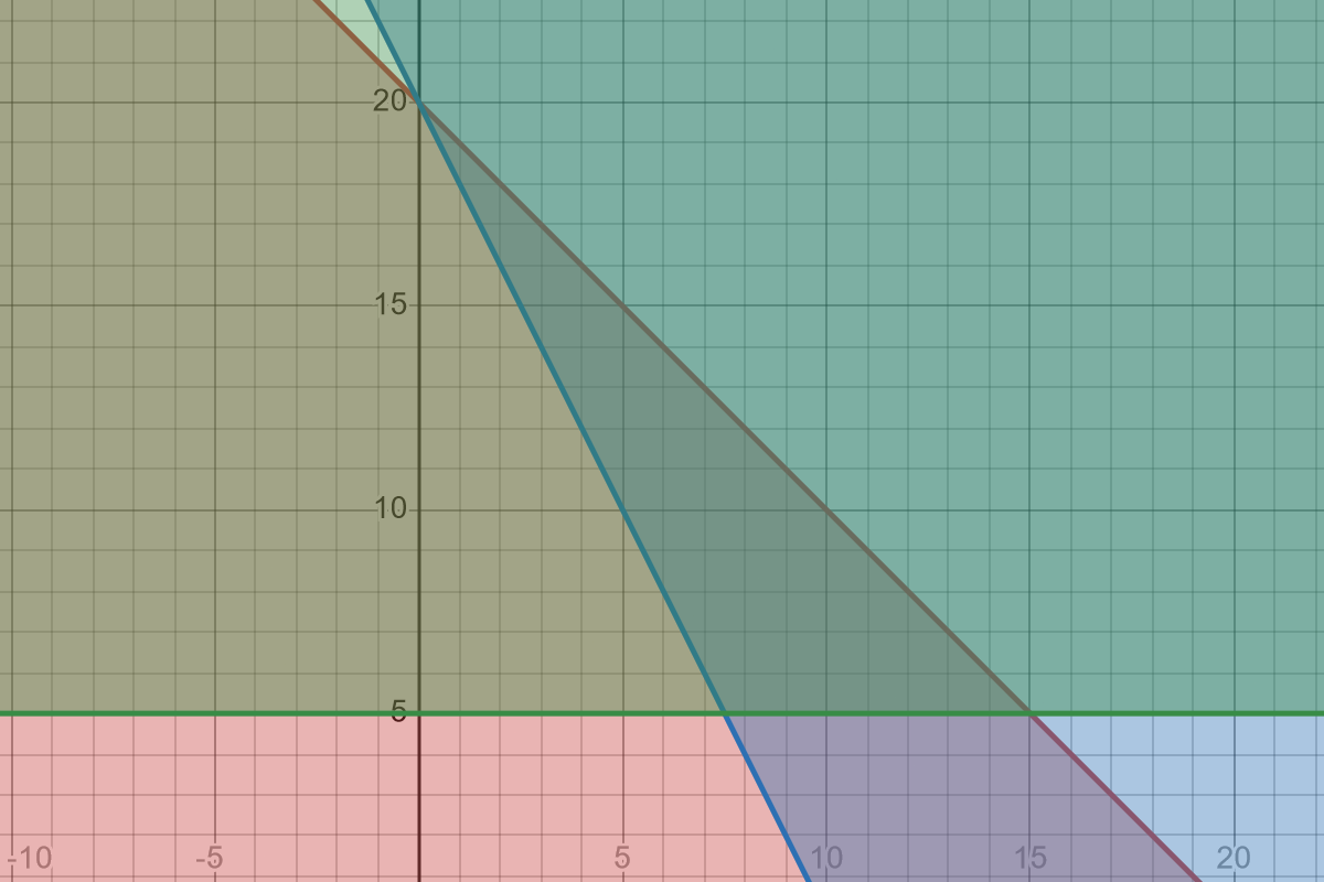
The triangle in the middle is where all three overlap, meaning any combination of hours in that region would satisfy all those restrictions. The three points of the triangle represent the extremes. One at $(0,20)$ for doing nothing by walking dogs, another at $(15,5)$ for mowing as much as possible, and the last at $(7.5,5)$ for working the fewest amount of hours he needs to work and still earn his \$200.
Three Variable Systems
We will go over these in class, and the book has the steps for one (here is a redone version of that example). For now, here are some guidelines for going about solving a three variable system, since taking the wrong steps can lead to dead ends. We’ll go over a more formal system next section.
- Eliminate the same variable from two of the equations.
- With those two equations down to two variables, solve that sub-system.
- Use your solutions to find the third value.
Writing Systems as Matrices
We’ve scratched the surface of a topic called linear algebra, a course some of you will run into in college. Linear algebra in an extension of solving systems, except of course, more complicated. Matrices are big part of this. For the moment, we’ll just learn to convert a system into a matrix and vice versa. Next section, we’ll do a bit more with matrices.
A matrix is just a rectangular array of numbers or symbols. Taking a system and writing it as a matrix means stripping out everything but the coefficients. The big catch is to make sure your equations are in standard form. So, all the variables on one side in alphabetical order, and the constant on the other side.
\[\left\{ \begin{aligned} 2x+3y&=1\\ 4x-2y&=10 \end{aligned}\right. \quad\Rightarrow\quad \left[ \begin{array}{cc|c} 2 & 3 &1 \\ 4 & -2 & 10 \end{array} \right]\]And if you are presented a matrix and need a system
\[\left[ \begin{array}{cc|c} 1 & 1 & 19 \\ 2 & 5 & 50 \end{array} \right] \quad\Rightarrow\quad \left\{ \begin{aligned} x+y&=19\\ 2x+5y&=50 \end{aligned}\right.\]Both matrices you see above are called augmented matrices, where the constants are present, but separated by a vertical line. A coefficient matrix has just the coefficients, but we won’t use them too often in this class.